
Guest blog post by R. Allan Reese
From the start, Downing Streets’ daily COVID press conferences have included various graphs slightly amended each day. In mid April on the Allstat list, I described the presentation and labelling of these graphs as “Boilerplate Excel” and was duly reprimanded for “slagging the people concerned off behind their backs” with “destructive criticism”. That was not my intention, nor do I accept that criticising a presentation equates with being derogatory about the author. I stand by the assertion that an equivalent lack of attention to spelling, grammar or punctuation would not be condoned in a PR organisation. The Downing Street presentations were not prepared by hard-pressed, front-line health staff, but by media-savvy folk around the PM. I wrote to the press office but received no response.
The basis for my criticisms comes from an approach I call Graphical Interpretation of Data (GID), expounded for example in various articles in Significance, freely available online. Number 10’s daily sequences of graphs and data are available at https://www.gov.uk/government/collections/slides-and-datasets-to-accompany-coronavirus-press-conferences.
It could be argued that changing a style of presentation risks accusations of “spin” if this detracts from the day-to-day comparison. However, some changes were made mid-stream. Initially, the daily numbers of deaths were plotted on a log scale labelled obscurely “5, 100, 2, 5, 1000, 2, 5, 10k” (Figure 1). The Daily Telegraph published a redrawn version labelling the grid line below the 5 with “0”. The label “5” actually meant 50 deaths to allow the trajectory for each country to be aligned from the day 50 deaths were reported. This is all very confusing.
Fig 1: 30 March. Early line graph with enigmatic Y labels and poor linkage to key.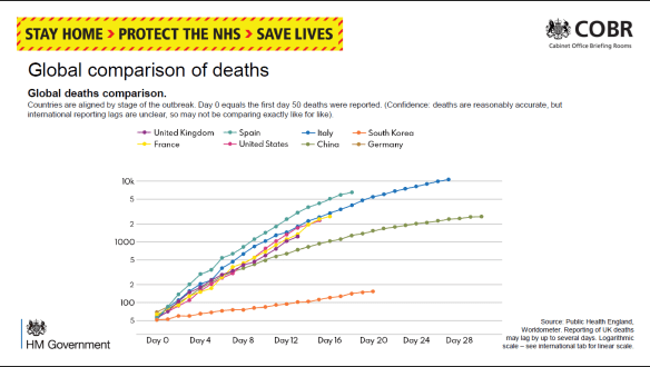
I wrote to the Telegraph about this, and their presentations improved, as did Number 10’s, with labels 50, 100, 200, 500, etc. The Metro commented on 1 April that the log scale made the growth in number of deaths appear less steep. They quoted David Spiegelhalter that each presentation has its “advantages and disadvantages” and “there is no ‘right’ way”. However, less mathematically-minded readers would surely see the choice and the changes as spin.
On 8 April these presentations switched to a linear scale with a scale labelled “2K, 4K, 6K …”, thus avoiding showing “real” numbers or a disturbing axis title “Thousands of deaths”. I described the use of ‘K’ as “nerdy”, especially as K in IT means a power of 2, not 1000. It is notable that the daily format of the press conferences was a speech by a minister who then handed over to a scientist or medic to describe the graphs, reinforcing the attitude that graphs are for “boffins” – they might be over your head, dear simple reader.
Within GID one often has to guess at the intention of the author: Was the choice of notation accidental or deliberate? Whom was this graph designed to inform? I think we have to assume the direct audience are journalists who then interpret the graphs and data for their readership. On the other hand, some features are so clearly defaults in spreadsheet graph production (e.g. text written horizontally or vertically), that I stand by the assertion that these presentations were handed out without further consideration or editing.
Downing Street’s daily “Global comparison of deaths” compares countries using a line chart. Initially the lines were just colour-coded with a separate key. Then the country names were written at the end of each line. Because each country’s “Day 0” was a different date, all the lines were different lengths. Because there were ten lines, some were difficult to identify, as some colours were very similar and there was no redundancy (variation in other line characteristics). The intended message appeared to be that the UK was buried in the middle, on a similar trajectory to the rest of Europe, with the US far worse (nearly three times as many deaths), while China and South Korea had fared much better.
It’s pretty obvious that crude numbers of deaths is a poor comparator, and there is much confusion between numbers of deaths and death rates. BBC’s More or Less (22 April) discussed this and identified the problem that converting using deaths per million population flung San Marino and Andorra to the top. But you have the same problem calculating rates for many statistics by London boroughs: Westminster may come out top because so few people live there but many people commute. The GID approach is to draw a graph (of numbers or rates), consider what message you wish to put across, and to revise the graph to clarify and emphasise.
Cristl Donnelly, on More or Less, suggested a better comparison would be to look at excess deaths in each country. This could also be standardised for population size, but might also allow a division into excess deaths from COVID and excess collateral deaths due to non-availability of other health services.
Another graph showed the number of deaths reported daily. In the first weeks this was for hospitals only, but from mid-April it showed Daily COVID-19 Deaths in All Settings. Note this was not necessarily the day the person died. Once the “peak” was passed, it was stressed in most presentations that there was a strong weekend effect with greater delays in reporting and hence a jump up each Monday. As a result the bar graph looks quite chaotic. A 7-day rolling average line clarified the general trend, but no visual effect was used to indicate weekends and the dates were labelled at 3-day intervals. Surely a good presentation would demonstrate the periodicity? (Fig 2)
Fig 2: 30 April. The bars show large day-to-day fluctuations while the smoothing line gives a clear, and more comforting, pattern. Which are weekends?
The other graph I draw attention to is the daily “New UK Cases”, based on the number of positive (PCR for antigen) tests reported that day (Fig 3). Initially this was constrained by test availability. By the third week of April a large excess of laboratory capacity over sampling numbers was reported. According to the rubric, “there are likely many more cases than currently recorded here”, predominantly because sampling was restricted to hospital patients and staff, then extended to wider NHS staff and care workers, but (at the time of writing) not to the wider population.
Fig 3: 19 April. The numbers written on bars were subsequently dropped as a separate data file was available. Without knowledge of the number of negative tests, it’s hard to evaluate any trend. 
Showing the number of positives against an increasing number of daily tests, but not showing the number of tests, disguises any trend in prevalence. It would help if the number of tests or the proportion positive were also reported; these might be split to show the proportions in groups showing symptoms (expected high) and those tested as contacts (hopefully, lower). Such comparisons were further hindered by gerrymandering the number of tests in late April to claim to have reached the arbitrary target of 100,000 tests “on” 30 April.
Among the problems with this chart are: the dates are written vertically with no indication of weekends or other divisions that might aid interpretation; the actual numbers are written on the bars, again vertically and hard to compare; for two thirds of the period shown the number varied between 4K and 6K and the largely overdrawn grid gives no assistance for comparison; most of the bars are split into two sections, linked to an enigmatic key (Pillar 1 and 2) which requires further recourse to the rubric for an explanation.
The split between “pillars” had me for one puzzled. It derived from the Secretary of State’s plan for five pillars of activity, but at various times the spokesmen distinguished the groups either by the targets for sampling (patients and hospital staff showing symptoms versus wider NHS staff and households) or by the place of testing (PHE versus commercial labs). I failed to find on the website any clear definitions to discriminate between “critical” and “key” workers. By the end of April this graph had become quite impossible to learn from: the number of cases detected by NHS labs was going down despite PHE opening its Lighthouse labs but the number from other mass testing (private) labs appeared to increase each day. Hence, it appeared to say nothing about the national prevalence and, since there was no effective treatment, offer no assistance to individual patients.
My interpretation is that this is a case of “reporting the data” out of a sense of duty or as a totem to show the approach is “scientific”. The layout obscures any visible trend except to show Pillar 2 as increasing over its range. High counts on 5 and 8 April are balanced by lows values on 4, 6 and 7 April, so a smoothing line would make the graph far easier to understand. Having so many written numbers makes this far more of a table than a graph; it’s no good on a screen, especially during a presentation, but you can print it and turn it sideways. Or you could opt for horizontal bars with time running down the screen; this layout fits less well on a landscape screen, but could be split into a row of panes by week.
For screen use, one could easily angle the dates, add grid lines or background shading for weekends and Easter, round the numbers and omit the commas, move the “6K” gridline to label the actual maximum and add a 5000 gridline, change “0K” to “0”, and make the key one-stage. As the interest is always in the latest figures, one could move the Y labels to the right-hand end. I would reconsider the colours: the orange is intrusive and a “warning” tint, and the blue is quite dark. Lighter, more neutral colours for the bars would go better with an overlain smoother.
None of this is rocket science or takes much time or resource, but it does show one has thought about the graph and the audience. It shows competence and consideration.